

Updated: 2026-11-07 By: Ari Heljakka
Short answer
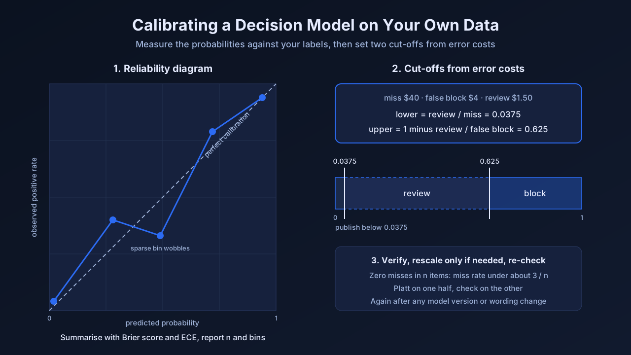
Label 100 to 200 items that look like your production traffic, run your exact questions over them, and check that the probabilities match what happened: items scored around 0.7 should be "yes" about 70 % of the time. Summarise with the Brier score and the expected calibration error (ECE). Pick two cut-offs from what each mistake costs: below the lower one act as "no", above the upper one act as "yes", and send the band in between to an LLM judge or a person. Rescale only if the check shows a consistent bias. Repeat the check whenever the model version or the question wording changes.
Calibrated questions are cheap enough to run on every conversation. Ask one narrow question per signal, store each answer as a score on the trace, track rates by topic and release, and send only the uncertain band to a slower judge.
Key facts
- Definition: A decision model is calibrated on your data when, among items it scores near 0.3, about 30 % are actually positive, and so on across the range. A conversation signal is a judgment read from the transcript, such as a correction or a request for a human.
- When to use: Before a probability triggers an automatic action or feeds a rate you report, and again after every model or wording change.
- Limitations: With 100 labels, calibration is only measurable in well-populated bins. Low cut-offs near 0.02 to 0.05 need many items in that region to verify.
- Example: A listing screen where a missed health claim costs $40, a wrong block $4 and a review $1.50 gets cut-offs of 0.0375 and 0.625, not 0.2 and 0.8.
- Jev 1.14: Released 2026-10-14; TypeSafe said
would move to it a week later. Our figures here come from
and have not been re-run on 1.14. - Last updated: 2026-11-07
Key takeaways
- "Trained for calibration" describes a training objective, not your data. Independent tests of Jev find good calibration on narrow factual yes/no questions and several times worse on subjective or rating tasks.
- Accuracy at 0.5 is the wrong summary for a model you will threshold. Read the reliability table and the Brier score.
- Thresholds follow from costs. Labels tell you whether the probabilities can carry them.
- A rescale fitted on a tiny set can make things worse. Fit on one half, check on the other.
- A successful outcome can hide a bad conversation. Score the conversation, one question per signal, and version the questions.
Definition
A probability is calibrated when it matches long-run frequency: of all items given 0.8, about 80 % turn out positive. This describes groups of predictions, not any single answer. Calibration is separate from discrimination. A model can rank items perfectly (high AUROC) and still be overconfident, and a model that always outputs the base rate is perfectly calibrated and useless. Discrimination decides how much traffic you can route automatically; calibration decides whether a cut-off means what you think.
Calibrating a decision model means measuring how well its probabilities match your labels, choosing thresholds from error costs, and only if needed fitting a small correction (a rescale). Thresholds are a policy choice. The measurement is evidence about one question version, one model version and one label set, and it only counts on rows not used to write or tune the question.
A decision model takes a state and typed questions and returns a probability per question, with no generated text. For question types and how probability differs from confidence, see what is a decision model.
Conversation signals are one place where calibrated probabilities pay off:
| Signal kind | Example | Coverage | Cost to collect |
|---|---|---|---|
| Explicit | Thumbs up or down, a star rating | Low, a few percent of users | Free |
| Behavioural | User closes the chat, abandons the flow | Full, but ambiguous | Free |
| Outcome | Payment completed, ticket closed, card unlocked | Full, but late and coarse | Free once instrumented |
| Conversation | User corrects the assistant, asks for a human | Full, if you can afford it | One evaluation per thread |
Only conversation signals say what went wrong inside the dialogue. "Card unlocked" is a success, yet the transcript may show a wrong instruction, a correction and a request for a person.
When this matters
- A probability drives an action with no human in between: blocking, approving, paging, refunding.
- You run a cascade, and the band boundaries between the decision model and an LLM judge are calibration decisions.
- Your domain differs from public benchmarks. Independent ECE measurements of Jev range from about 0.011 on factual claim checks to 0.284 on answer rating.
- The wording changed or the model alias moved, and you need to know whether last month's thresholds still hold.
- Sampling hides rare failures. If 2 % of conversations end with a hand-off request and you judge a 1 % sample of 10,000 daily threads, you see about two a day.
- Outcome metrics lag. A rise in corrections can show up within hours of a prompt or model change.
It matters less if you can read every conversation, already collect rich explicit feedback, or need an open-ended judgment.
How it works
The procedure in brief:
- Label 100 to 200 items that look like your real traffic. Split them into a tuning half and a check half.
- Run your exact questions on a pinned model version and record each probability.
- Group the items by predicted probability (0 to 0.1, 0.1 to 0.2, and so on) and count how often each group is actually "yes". Items scored around 0.7 should be "yes" about 70 % of the time.
- Summarise with the Brier score and ECE, on the check half only.
- Pick two cut-offs from what a miss, a false block and a review each cost.
- Rescale only if the groups show a consistent bias.
- Repeat when the model version, wording, label definition or traffic changes.
Step 1: Build the label set
Size. 50 to 100 items is the usual starting point. It shows gross miscalibration and lets you compare two wordings, but cannot verify a cut-off in the tails. If a bin holds n items and none is a miss, the 95 % upper bound on the miss rate is roughly 3 divided by n (the "rule of three"). To show that items below 0.04 are positive less than 4 % of the time, you need about 75 items in that bin alone. Plan for 100 to 200, more if positives are rare.
Composition. Draw most items at random from production. If positives are rare (a 2 % rate leaves 2 positives in 100), add an enriched sample from a keyword search or past flags, and record a sampling weight per item so you can reweight to production rates. Without reweighting you measure the enriched set, not production. Add near-boundary cases and documented weak spots; for Jev these are counting, numeric and date comparison, multi-hop reasoning and double negation.
Labels. Write a one-paragraph definition of "positive" first. Have two people label 30 to 50 items independently. Their disagreement rate is the noise floor.
Split. Tune on the first half (wordings, few-shot examples, cut-off search, rescale). Report from the second. If you reword after seeing results on the second half, it has become tuning data. Below about 100 items, use cross-validation.
Step 2: Run the exact questions
Use the production question text,
Step 3: Read the reliability diagram
Sort items into ten equal-width bins. Plot mean predicted probability against observed positive rate, with counts. Calibrated points sit on the diagonal. Below it at the top and above it at the bottom means overconfidence, the typical failure Guo et al. (2017) documented for modern neural networks. Points on one side mean a bias.
Read the counts first. In our run at Scorable on 200 HaluEval-QA items with
Step 4: Summarise with Brier score and ECE
The Brier score (Brier, 1950) is the mean squared difference between probability and the 0 or 1 label; lower is better. Compare it with always predicting the base rate b, which scores b times (1 minus b). It rewards calibration and discrimination together, so it is the best single number for comparing two questions.
The expected calibration error (Naeini et al., 2015) is the count-weighted average gap between predicted and observed rate across bins. It isolates calibration, but depends on the bin count and is biased upward on small samples. Report bins, n, and the question, model and label versions with it.
What to expect: we measured ECE 0.037 (10 bins, n = 200) on HaluEval-QA, and a third-party test on 88 relabelled HaluEval items found a Brier score of 0.043 for Jev against 0.054 for an LLM judge whose stated confidence took only six distinct values. HaluEval may be in the training data, so treat both as upper bounds. Independent studies spread wider: ECE 0.012 to 0.046 on police crash narratives (Rafe and Das, 2026) and 0.011 on claim verification (Vals.ai), but 0.108 on LegalBench (Vals.ai), a median of 0.157 over 15 social-science annotation tasks (Ibrahim and Zaki, 2026) and 0.284 on HelpSteer2 answer rating (AI/ML API). TypeSafe publishes no figure, and its documentation says score levels are "weak in numerical calibration".
Step 5: Choose two thresholds from error costs
Three actions: let through, review, block. Assign costs:
- c_miss: a positive you let through.
- c_false_block: a negative you blocked.
- c_review: one review by an LLM judge or a person, assumed correct.
If p is calibrated, letting an item through costs p × c_miss on average, blocking costs (1 minus p) × c_false_block, and reviewing costs c_review. The cheapest action gives:
- lower cut-off = c_review / c_miss
- upper cut-off = 1 minus c_review / c_false_block
If the lower comes out above the upper, review never pays; use one cut-off at c_false_block / (c_miss + c_false_block).
The vendor documentation uses 0.2 and 0.8 as an example and advises raising the threshold when a false yes is costly. The formula makes that numeric. In our HaluEval-QA run, the 0.2 to 0.8 band decided 80 % of items at 95.0 % accuracy; 0.05 to 0.95 decided 62 % at 97.6 %. That is the trade-off you are pricing.
Also run an empirical cost-minimising search on the tuning half, as a cross-check only: on small sets the optimum lands on data points and its cost is optimistic. If formula and search disagree badly, the probabilities are probably off in that region.
Step 6: Rescale only when the diagram says so
If the diagram shows a consistent shape and you have enough labels, fit a correction on one half and check it on the other. It can help a lot: in the crash-narrative study, a simple recalibration cut calibration error by a factor of 3.3.
- Platt scaling (Platt, 1999) fits a two-parameter logistic regression on the log-odds. Temperature scaling, the one-parameter variant Guo et al. (2017) recommend, fixes the bias at zero. Both suit fewer than a few hundred labels.
- Isotonic regression (Zadrozny and Elkan, 2002) fits any monotone step function, but needs several hundred labels to beat Platt.
Tiny sets overfit. On a readability rubric we fitted a linear rescale of
Step 7: Re-check on every change
- Model version.
moves with each release. TypeSafe advises sending a versioned ID (such as
, reported in every response's
field) once thresholds are tuned. Every threshold here was measured on 1.13. TypeSafe promises 60 days' notice before retiring
; plan the re-check rather than wait. - Question wording. One question design gave held-out error from 0.038 to 0.079 depending only on level wording, and few-shot examples helped one wording and hurt another.
- Label definition. New definition, new check.
- Input distribution. A new category, language or upstream model shifts the base rate. Re-sample periodically.
Decision models are near-deterministic: our repeat standard deviation for Jev was 0.001 to 0.004, against 0.009 for an LLM judge. A shift after a change is the model, not noise. The flip side: asking twice gives no second opinion.
Choice and score questions
For
Example: calibrating a health-claim screen
A marketplace must keep listings from claiming a product treats, cures or prevents a disease. A missed claim is priced at $40 of regulatory exposure, a wrongly blocked listing at about $4, a human review at $1.50. About 3 % of listings contain such a claim.
The response carries the answering version and the probability, here
Label set. 120 random listings (about 4 positives) plus 60 matching "cure", "immune", "prevent" or "clinically" (about half positive), each enriched item weighted down to its production share.
Thresholds. Lower 1.50 / 40 = 0.0375; upper 1 minus 1.50 / 4 = 0.625. The band is lopsided because a miss costs ten times a false block. At a $3.00 review cost the cut-offs move to 0.075 and 0.25; at $4.00 or more review never pays and one cut-off at 4 / 44, about 0.09, is optimal.
Verification. The lower cut-off carries the risk. For weighted items, replace n in the rule of three with the effective sample size n_eff = (sum of weights)² / (sum of squared weights). Say 90 items fall below 0.0375 with no positives: 60 random at weight 1, 30 enriched at weight 0.1. Then n_eff is 63² / 60.3, about 66, and the bound is about 4.6 %, above the 3.75 % the cut-off assumes. Not verified yet: it needs n_eff of 80, about 15 more random items in that region. Any positive below the cut-off means label more there or lower it.
On 200 simulated items drawn from perfectly calibrated probabilities, the empirical search returned about 0.09 and 0.55 against the formula's 0.0375 and 0.625. That is the noise a 200-item search carries.
Using calibrated questions to catch conversation signals
A decision model answers a set of signal questions about a whole conversation in one call, typically in under half a second for a fraction of a cent, so you can score every conversation. The steps above decide which scores you can act on.
Pick signals someone will act on
A signal earns its place if a rising rate would trigger a specific change:
| Signal | Question type | Stored as | Who acts on it |
|---|---|---|---|
| Topic | | Categorical label | Used to slice every other signal |
| Frustration | | Numeric, expected level, 0 to 1 | Conversation design, escalations |
| Correction | | Numeric, P(true) | Prompt and knowledge-base owners |
| Repeated request | | Numeric, P(true) | Intent handling, flow design |
| Hand-off request | | Numeric, P(true) | Support staffing, coverage gaps |
| Out-of-scope ask | | Numeric, P(true) | Product scope, compliance |
| Resolution claimed | | Numeric, P(true) | Cross-check against outcome events |
Write narrow questions and score once per conversation
- One condition per
. "Frustrated and asks for a human" is two questions; combine them in code. - Phrase it so a high value means yes. "The conversation is free of corrections" can be read backwards.
- For
, describe concrete situations per level, not degrees such as "moderately frustrated". - For
, include an
option. - Avoid counting. Ask "the user repeats a request the assistant had not handled", not "asked three or more times", and trim banners and tool payloads, since TypeSafe says irrelevant context degrades accuracy.
Score when the conversation closes or goes idle. One call covers all seven questions, answered in parallel against the same state. Turn-level signals are different questions and cost a call per turn.
Store each answer as a score on the trace
An evaluation or observability platform can keep each answer as a score on the trace, next to LLM-judge and code-evaluator scores. A
Example: a card declined abroad
The outcome event says the card was unblocked. The transcript tells a different story.
Illustrative answers (they show the shape, not a measurement): topic
So: resolved, but with a confident correction and an out-of-scope ask, frustration between mild and complaining, and two signals in the uncertain band. "Repeat" is ambiguous because the user restated a fact, not a request. "Hand-off" is ambiguous because the user asked for a person next time. Both deserve a second opinion and raise a wording decision: should a future-tense hand-off count? Write the answer into the
Rates: expected count, not just a threshold count
Scores find threads; rates decide things. A thresholded rate (share above a cut-off) is easy to explain but discards the probabilities and jumps when many threads sit near the cut-off. An expected rate (mean probability) is unbiased if the model is calibrated on this traffic, and moves smoothly. This is where Steps 1 to 4 pay off. Report both. A gap between them can mean many moderate probabilities away from the cut-off, or miscalibration, not only ambiguity, so plot the distribution before concluding.
The last column is what outcome metrics miss: conversations that ended well after the assistant got something wrong. A stale knowledge-base article shows up there first. The combined rule is not calibrated just because its inputs are; both read the same transcript, so their errors correlate. Label a sample for it before quoting it as a rate.
Alerts: change against a baseline, sliced by topic
Absolute thresholds ("alert above 5 % hand-offs") break when the traffic mix shifts. Compare each slice with its own recent baseline and require a minimum volume:
Because scores are near-deterministic (Step 7), a rate change is traffic, not evaluator noise, and a rewording moves the baseline. Never compare rates across question versions. Split by release too: a correction rate that doubles the day a prompt ships is a regression; the same rise across all releases is more likely a change in what customers ask.
Sample the uncertain band
The decision model decides where the LLM judge and people look:
- Confident yes on hand-off, correction or out-of-scope goes straight to the owner's queue.
- Uncertain band, or a
or
confidence below 0.5, goes to an LLM judge whose verdict and reason a reviewer can read. - Still unclear or consequential cases, plus a small random sample of everything, go to a person. The random sample tells you whether the confident decisions are right.
The 0.2 to 0.8 split that decided 80 % of items was measured on HaluEval, a hallucination task. We carried those thresholds over to conversations without measuring them on conversation data, so measure the split on your transcripts before sizing the judge budget. Name the judge's model, too: on a readability-ordering task the same rubric scored 0.786 pairwise accuracy on a gpt-4o-class model and 0.964 on gpt-5.5.
The human labels become your conversation calibration set. Fifty to a hundred held-out conversations per signal, not used to write the question, is enough for a reliability check as in Step 3. On the same rows, ask the LLM judge the same question and compare agreement with the labels (accuracy or Cohen's kappa) signal by signal. Where the decision model agrees less, route that signal to the judge or rewrite the question.
Cost at full traffic
TypeSafe lists Jev at $0.042 per million input tokens, output free. A 1,500-token transcript costs about $0.00006 for all seven questions, about $6 a day at 100,000 conversations. On shorter items we measured about $0.000022 per evaluation at a typical median latency of 0.42 s (indicative; it varies with region, payload and load). An LLM judge also bills output and takes seconds per call, so it usually runs on a sample. For accuracy against LLMs, see decision model vs LLM accuracy on scoring and classification.
Comparison
| Criterion | Sampled LLM judge | Decision model on every thread | Decision model plus judge on uncertain band |
|---|---|---|---|
| Coverage | Sample, often 1 to 10 % | All conversations | All conversations |
| Per-signal output | Verdict and reason | Probability or label | Probability, plus reason where uncertain |
| Rare-signal rates by topic | Noisy at small samples | Stable | Stable |
| Explains a single thread | Yes | No | Yes, for the threads that need it |
| Repeatability | Varies with model and temperature | Near-deterministic in our runs | Near-deterministic for most threads |
| Main risk | Missing rare failures | Silent miscalibration on your traffic | Thresholds drift after model or wording changes |
Limitations
- Small sets cannot verify tails. The cut-offs that matter most sit where you have fewest items. Budget labels there.
- Costs are guesses. Try a few plausible values and see whether the band moves enough to matter.
- Reviewers make errors. Measure the judge's two error rates separately, and per score band: how often it passes a real positive (e_miss, measured on positives) and how often it flags a negative (e_block, measured on negatives). An overall error rate is not enough. When positives are rare, a judge can miss most of them and still be right 90 % of the time overall. The expected cost of a review then becomes c_review + p × e_miss × c_miss + (1 minus p) × e_block × c_false_block, with the rates for the band the item falls in. Errors near a cut-off are usually higher than the class-wide average. It depends on p, so recompute both cut-offs against p × c_miss and (1 minus p) × c_false_block.
- Calibration depends on the task. Our figures and the third-party Brier scores come from HaluEval, which may be in the training data, and independent ECE for Jev ranges from 0.011 to 0.284 by task. The conversation-signal thresholds here are carried over from HaluEval, not measured on conversations.
- Calibration drifts. A reliability table describes one period's traffic, model version, wording and labels.
- Combined decisions need their own labels. Calibrated parts do not make a calibrated whole. Label the final action and measure it.
- No rationale. You learn that a conversation contained a correction, not which turn, and not why a slice is miscalibrated. The usual fix is splitting or rewording, then a fresh check.
- Long transcripts. TypeSafe documents a 64k-token request limit and 32k per question; an opt-in long-context header raises both to 262k, with lower accuracy. Strip boilerplate and split long threads.
- Language. Jev is English-first by TypeSafe's description. TypeSafe expects the largest 1.14 gain in multilingual support; test it per language.
- Prompt injection. TypeSafe says the model is not robust to instructions injected into the state, and transcripts contain user text. Do not let a signal gate anything a user could profit from gaming without a second check.
- Signals are not outcomes. More hand-off requests may be good news if a human-support option just launched. Read rates next to the change log.
Evidence and sources
Evidence:
- Product docs: TypeSafe, Confidence; Noul, Score and Choice questions (response shape, phrasing rules, threshold guidance, expected-level score, the
option) - Third-party benchmark (88 HaluEval items, Brier 0.043 vs 0.054, run 2026-09-21): OpenRouter, Jev vs LLM-as-a-Judge
- Independent calibration studies: Rafe and Das, 2026, police crash narratives, arXiv:2609.24052; Ibrahim and Zaki, 2026, 15 social-science annotation tasks, arXiv:2609.24574; Vals.ai, Independent evaluation of Jev; AI/ML API, What is Jev
- Our measurements: HaluEval-QA English, n = 200,
, run 2026-09-19 (accuracy 0.880, AUROC 0.956, ECE 0.037, reliability groups, cascade bands, median 0.42 s, cost); readability rubric, 8 dev and 8 held-out items, run 2026-09-20 (rescale, wording sensitivity, judge-model comparison, repeat variance). Not re-run on
. Methodology write-up pending. - Updated: 2026-11-07
Further sources:
- TypeSafe, "Jev: For the builders AND dreamers" (Jev 1.14 release post), 2026-10-14, and the Jev models page, for the 1.14 release, long context and the
alias. - TypeSafe, Jev introduction and early-access announcement, 2026-09-15, for pricing, request limit, language support and documented weaknesses.
- TypeSafe, model jaggedness, for "weak in numerical calibration" and the documented weak spots; "Machine learning primer", for the group-level definition of calibration.
- Brier, G. W., 1950, "Verification of forecasts expressed in terms of probability", Monthly Weather Review.
- Platt, J., 1999, "Probabilistic Outputs for Support Vector Machines and Comparisons to Regularized Likelihood Methods".
- Zadrozny, B. and Elkan, C., 2002, "Transforming Classifier Scores into Accurate Multiclass Probability Estimates", KDD.
- Naeini, M. P., Cooper, G. F. and Hauskrecht, M., 2015, "Obtaining Well Calibrated Probabilities Using Bayesian Binning", AAAI.
- Guo, C., Pleiss, G., Sun, Y. and Weinberger, K. Q., 2017, "On Calibration of Modern Neural Networks", arXiv:1706.04599.
- Li et al., 2023, "HaluEval: A Large-Scale Hallucination Evaluation Benchmark for Large Language Models", arXiv:2305.11747.
FAQ
How many labelled items do I need? 50 to 100 shows gross miscalibration. To verify a low cut-off, count the items below it: with none positive, the miss rate is bounded at about 3 divided by that count. Most teams end up at 100 to 200. For conversation signals, size the set by positives, not conversations. A signal in 1 % of conversations leaves a random sample of 100 with no positives about a third of the time, and no sample like that can check calibration. Add an enriched sample with sampling weights until each signal has at least 20 to 30 positives, and report an interval with each probability range, not just its point estimate.
Is Jev calibrated out of the box? On narrow factual yes/no questions, independent tests find ECE of about 0.01 to 0.05. On subjective, legal or rating tasks it is several times worse, up to 0.284. TypeSafe publishes no figure. A simple recalibration cut error 3.3 times in one study.
Should I use ECE or the Brier score? Both. Brier to compare candidate questions, ECE and the reliability diagram to see where probabilities are off. Report n and the bin count.
Are 0.2 and 0.8 good default thresholds? No, they are a documentation example. Compute cut-offs from the cost of a miss, a false block and a review. With asymmetric costs the band is lopsided.
Do I need to recalibrate when the model updates? Yes. Pin the reported version, re-run your labels on the new version before moving the pin, and recompute thresholds. Same after any rewording.
Why not just use an LLM judge for conversation signals? Its cost and latency usually limit it to a few percent of traffic, which makes rare signals noisy per topic. A decision model covers everything and the judge reads the uncertain conversations.
Related reading
- What is a decision model?
- Decision model vs LLM: accuracy on scoring and classification, and when to use each
- How to read and interpret classical LLM metrics vs. LLM-judge metrics
- How do you run a human-aligned LLM evaluation workflow in production?
- How do you evaluate multi-turn agent conversations?
- What metrics, alerts, and reliability checks belong in an agent monitoring playbook?